RANDU example

This example is adapted from Tyler et al. (2009) and illustrates the behavior of ICS on data generated by the well-known RANDU pseudo-random number generator.

The way in which RANDU generates its numbers is somewhat deterministic. Upon closer inspection, a structure can be seen in the data, which becomes clearer when the ICS method is applied. The example highlights how ICS is able to identify informative directions associated with these dependencies, in contrast to variance-based approaches such as PCA.

from icspylab import ICS, plot_ics
from icspylab.distributions import generate_randu
from sklearn.decomposition import PCA
from sklearn.preprocessing import StandardScaler
import matplotlib.pyplot as plt

The dataset is generated using the icspylab.distributions.generate_randu() function.

X = generate_randu()
print("X shape:", X.shape)

X shape: (400, 3)

The plot below illustrates the generated RANDU dataset in three dimensions.

fig = plt.figure()
ax = fig.add_subplot(projection="3d")
ax.scatter(X[:, 0], X[:, 1], X[:, 2], s=2)
plt.show()

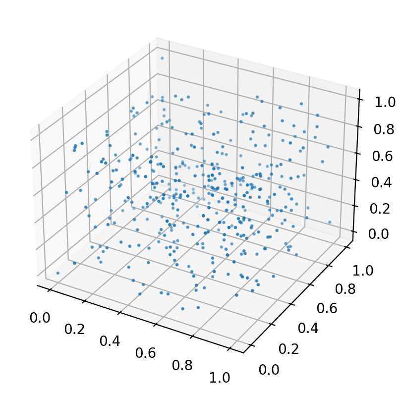
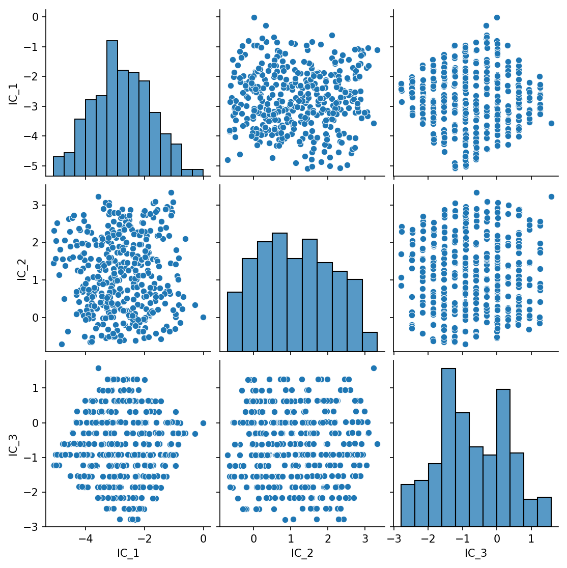
In three-dimensional space, each point represents 3 consecutive pseudorandom values, and it is known that these points fall in one of 15 two-dimensional planes. Applying ICS yields the following invariant components, which clearly exhibit those planes on the last component.

ics = ICS(S1="cov", S2="tcovAxis", algorithm="standard")
X_ics = ics.fit_transform(X)
plot_ics(X_ics)

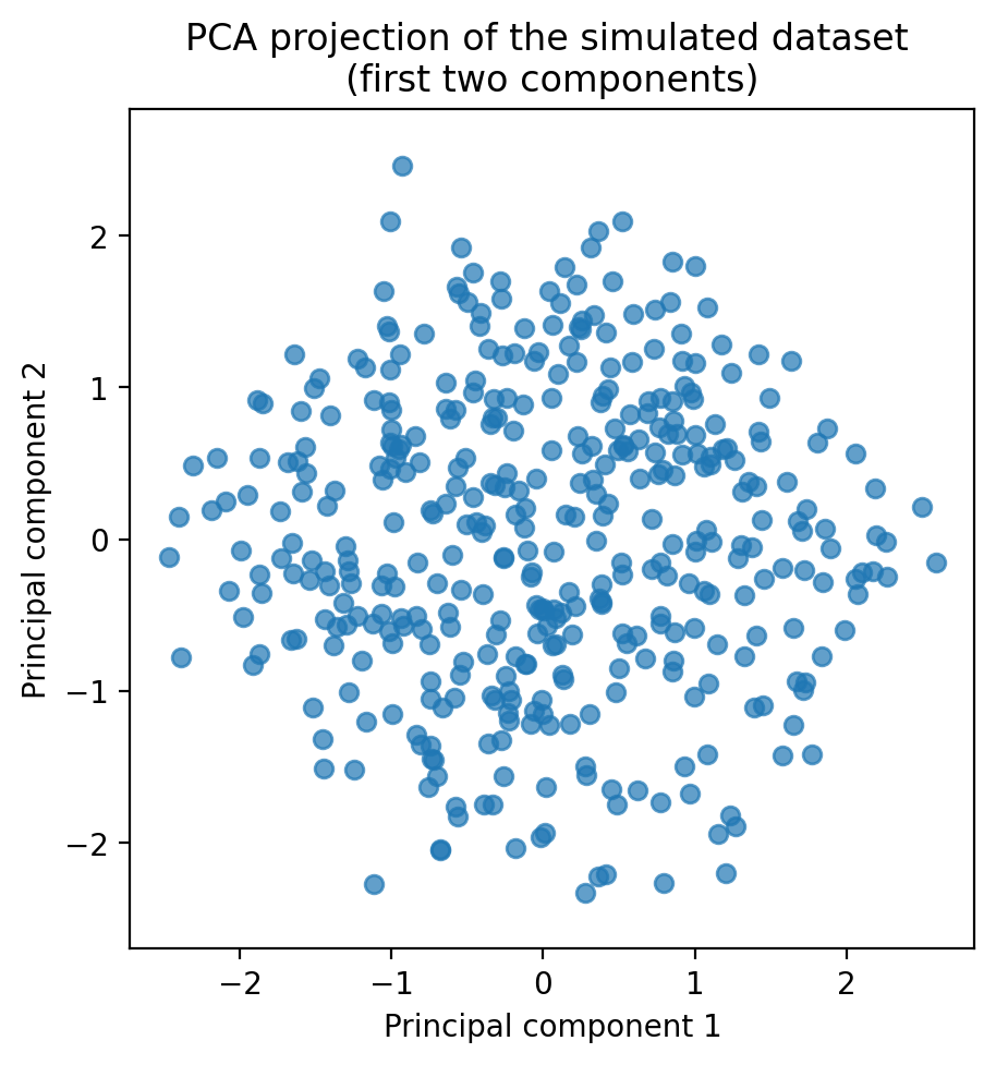
On the contrary, the underlying structure of RANDU is not visible on the first principal components.

# Compute the principal components
scaler = StandardScaler().set_output(transform="pandas")
X_scaled = scaler.fit_transform(X)

pca = PCA(n_components=2)
X_pca = pca.fit_transform(X_scaled)

# Plot the principal components
plt.figure(figsize=(5, 5))
plt.scatter(X_pca[:, 0], X_pca[:, 1], alpha=0.7)
plt.title("PCA projection of the simulated dataset \n(first two components)")
plt.xlabel("Principal component 1")
plt.ylabel("Principal component 2")
plt.axis("equal")
plt.show()