Clustering

In this example, ICS is used for exploratory data analysis. Using a real-world dataset, it illustrates how ICS can reveal interesting structures in the data - in this case, clusters.

The dataset used here is the same as in the Outlier Detection tutorial, namely the Forest covertypes dataset. It contains cartographic information about forest patches, where the target variable corresponds to the dominant tree species in each patch. The dataset includes 54 features whose description is available online.

This example focuses on exploratory analysis of the observations belonging to cover type 2, which is the largest class in the dataset.

First, let us load the dataset, separate the features X and the target y, and filter the observations corresponding to cover type 2 (y=2).

from sklearn.datasets import fetch_covtype

X, y = fetch_covtype(return_X_y=True, as_frame=True)
print(y.value_counts())
s = (y == 2)
X = X.loc[s]
y = y.loc[s]

print("X shape:", X.shape)

Cover_Type
2    283301
1    211840
3     35754
7     20510
6     17367
5      9493
4      2747
Name: count, dtype: int64

X shape: (283301, 54)

As in the Outlier Detection example, we remove variables containing almost only zeros in order to avoid singularity issues.

# Features cleaning
zero_ratio = (X == 0).mean()
cols_to_drop = zero_ratio[zero_ratio > 0.95].index
print("Features to drop (more than 95% of 0 values):\n", cols_to_drop)
X = X.drop(cols_to_drop, axis=1)
print("X shape:", X.shape)

Features to drop (more than 95% of 0 values):
 Index(['Wilderness_Area_1', 'Wilderness_Area_3', 'Soil_Type_0', 'Soil_Type_1',
       'Soil_Type_2', 'Soil_Type_3', 'Soil_Type_4', 'Soil_Type_5',
       'Soil_Type_6', 'Soil_Type_7', 'Soil_Type_8', 'Soil_Type_9',
       'Soil_Type_10', 'Soil_Type_12', 'Soil_Type_13', 'Soil_Type_14',
       'Soil_Type_15', 'Soil_Type_16', 'Soil_Type_17', 'Soil_Type_18',
       'Soil_Type_19', 'Soil_Type_20', 'Soil_Type_21', 'Soil_Type_23',
       'Soil_Type_24', 'Soil_Type_25', 'Soil_Type_26', 'Soil_Type_27',
       'Soil_Type_30', 'Soil_Type_33', 'Soil_Type_34', 'Soil_Type_35',
       'Soil_Type_36', 'Soil_Type_37', 'Soil_Type_38', 'Soil_Type_39'],
      dtype='str')
X shape: (283301, 18)

Since the dataset contains more than 280,000 observations, we keep only 5% of the data to reduce the computational cost.

# Subsample the data
X_sub = X.sample(frac=0.05, random_state=42)
print("X_sub shape:", X_sub.shape)

X_sub shape: (14165, 18)

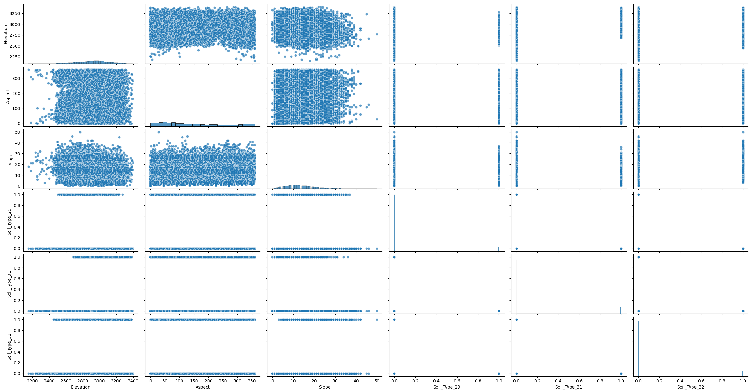
When looking at the original data, no clear structure is visible. We therefore apply dimensionality reduction to better reveal any underlying organization.

from icspylab import plot_ics

plot_ics(
    X_sub,
    col_names=X_sub.columns.tolist(),
    plot_kws={'alpha':0.7}
)

PCA

We begin by applying PCA for dimensionality reduction and visualizing the resulting principal components. Although all components are retained, only the first six are shown for readability.

from sklearn.preprocessing import StandardScaler
from sklearn.decomposition import PCA

scaler = StandardScaler().set_output(transform="pandas")
scaled_X_sub = scaler.fit_transform(X_sub)

pca = PCA()
X_transformed_pca = pca.fit_transform(scaled_X_sub)

plot_ics(
    X_transformed_pca,
    components="first",
    col_names=[f"PC_{i+1}" for i in range(X_transformed_pca.shape[1])],
    plot_kws={'alpha':0.7}
)

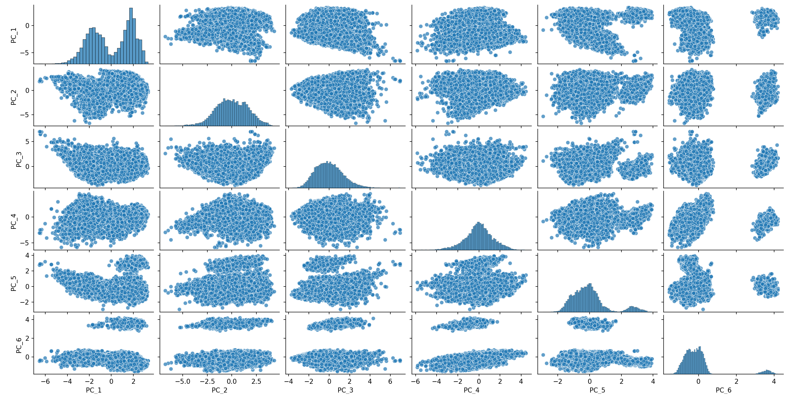
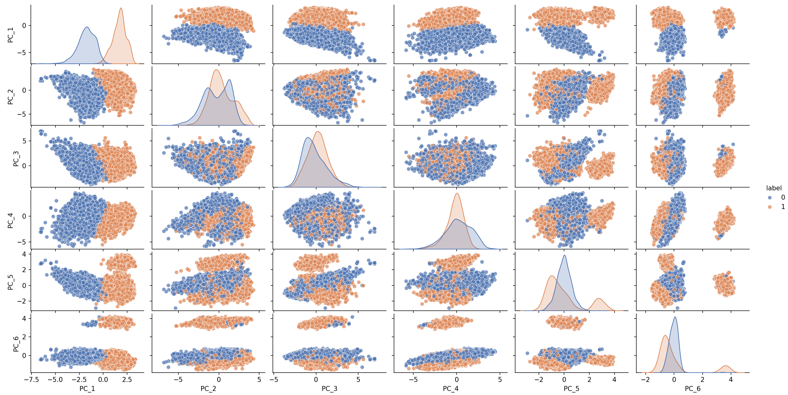
The first components reveal 2 clusters. Some structure is also visible on IC5 and IC6, each isolating a cluster and some seems overlapping in the main bulk. As an illustration, we apply KMeans with n_clusters=2.

from sklearn.cluster import KMeans

kmeans_pca = KMeans(n_clusters=2, random_state=0, n_init="auto").fit(X_transformed_pca)
plot_ics(X_transformed_pca, y=kmeans_pca.labels_,
         components="first",
         col_names=[f"PC_{i+1}" for i in range(X_transformed_pca.shape[1])],
         plot_kws={'alpha':0.7})

ICS

We apply the same methodology using ICS in place of PCA. The invariant components are computed and visualized. As in PCA, all components are retained.

from icspylab import ICS

ics = ICS(S1="tcov", S2="cov", center=True)
X_transformed_ics = ics.fit_transform(X_sub)
plot_ics(X_transformed_ics, components="first", plot_kws={'alpha':0.7})

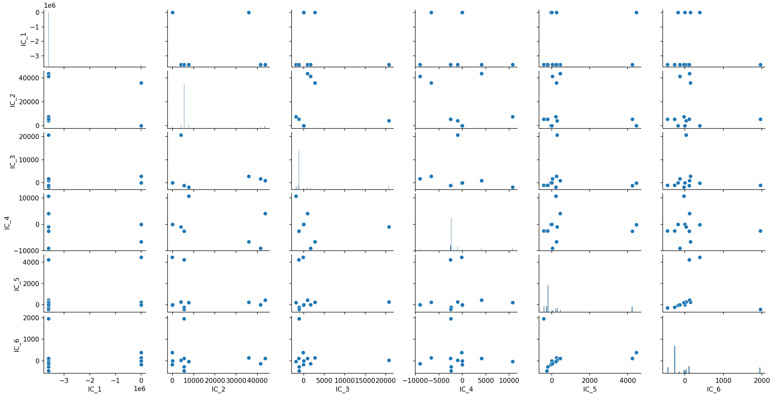
The IC_2–IC_3 projection reveals a clear clustered structure, with roughly seven visually distinct groups. We therefore apply KMeans with n_clusters=7.

kmeans_ics = KMeans(n_clusters=7, random_state=0, n_init="auto").fit(X_transformed_ics)
plot_ics(X_transformed_ics, 
         components="first", 
         y=kmeans_ics.labels_, 
         plot_kws={'alpha':0.7})

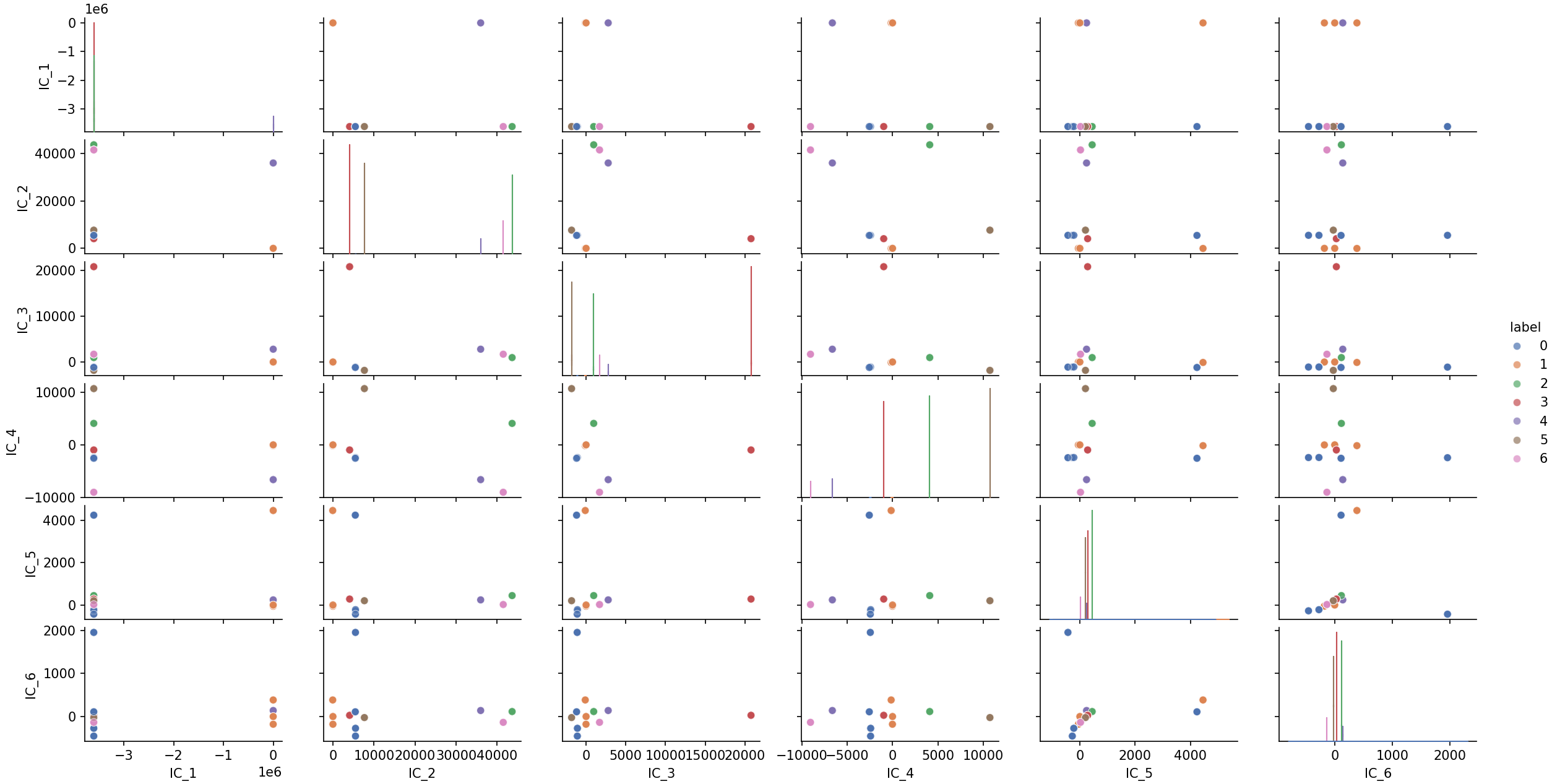
While PCA mainly highlights two broad groups, ICS reveals a richer cluster structure that becomes visible in only a few components. This illustrates how ICS can help uncover meaningful subgroups during exploratory data analysis.