Outlier detection

This example illustrates how ICS can serve as an effective preprocessing step for outlier detection. ICS constructs a new coordinate system in which anomalous observations become more separated from the bulk of the data. By concentrating non-Gaussian structures into specific invariant coordinates, ICS can make anomalies more visible and therefore easier to detect using standard outlier detection algorithms. In some cases, removing invariant coordinates associated mainly with noise can further improve outlier detection performance.

The problem we consider comes from scikit-learn’s Evaluation of outlier detection estimators example. The dataset is the Forest covertypes dataset, which contains observations describing forest patches together with the dominant tree species for each patch. It includes 54 features whose description is available online. Originally, predicting the target variable is a multiclass classification problem with 7 covertypes.

Following the methodology of scikit-learn’s example, we adapt the dataset into an outlier detection problem by considering observations with label 2 as inliers and observations with label 4 as outliers. This setup creates a highly imbalanced problem with a clear distinction between a dominant class and rare anomalies, which is well suited to evaluate outlier detection methods. The outlier detection algorithms considered here are Local Outlier Factor (LOF) and Isolation Forest (IForest).

In this tutorial, we reproduce the scikit-learn example and extend it by introducing an ICS preprocessing step before applying LOF and Isolation Forest. The goal is to assess whether expressing the data in ICS coordinates, and optionally removing invariant coordinates associated mainly with noise, improves the detectability of outliers compared with the original feature space. This example also demonstrates how easily ICS can be integrated into a standard machine learning pipeline.

First, let us import the dataset, separate the features X and the target y and encode the inliers (y=0) and outliers (y=1) to follow scikit-learn’s evaluation conventions.

import numpy as np
from sklearn.datasets import fetch_covtype

X, y = fetch_covtype(return_X_y=True, as_frame=True)
s = (y == 2) + (y == 4)
X = X.loc[s]
y = y.loc[s]
y = (y != 2).astype(np.int32)

print("X shape:", X.shape)

X shape: (286048, 54)

The features contain a lot of dummy variables Soil_Type. The exploration of the features reveals that many of them contains almost only zeros. Such features may lead to nearly singular scatter matrices, which can affect the eigen decomposition underlying ICS. We decide to drop them to avoid any issues.

# Features cleaning
zero_ratio = (X == 0).mean()
cols_to_drop = zero_ratio[zero_ratio > 0.999].index
print("Features with more than 99.9% of 0 values:\n", cols_to_drop)
X = X.drop(cols_to_drop, axis=1)
print("X shape:", X.shape)

Features to drop (more than 99.9% of 0 values):
 Index(['Soil_Type_0', 'Soil_Type_4', 'Soil_Type_6', 'Soil_Type_7',
       'Soil_Type_13', 'Soil_Type_14', 'Soil_Type_20', 'Soil_Type_34',
       'Soil_Type_35', 'Soil_Type_36'],
      dtype='object')
X shape: (286048, 44)

As the dataset contains over 280,000 samples, we subsample it to reduce the computational cost while maintaining class imbalance. We select 5% of the samples for training and 5% for testing.

from sklearn.model_selection import train_test_split

# Train test split
X_train, X_other, y_train, y_other = train_test_split(X, y, train_size=0.05, stratify=y, random_state=42)
X_test, _, y_test, _ = train_test_split(X_other, y_other, train_size=0.05, stratify=y_other, random_state=42)

n_samples, n_features = X_train.shape
anomaly_frac = y_train.mean()
print(f"{n_samples} datapoints with {y_train.sum()} anomalies ({anomaly_frac:.02%}) and {n_features} features")

14302 datapoints with 137 anomalies (0.96%) and 44 features

The training set contains approximately 0.96% anomalies, reflecting a highly imbalanced detection problem. Let’s see how LOF and IForest are performing to identify them and if their performance improves if we apply them on the invariant coordinates instead of the original features.

LOF

The first pipeline is LOF without ICS. Since LOF is distance-based, the data must be properly scaled. We therefore include a preprocessing step using a RobustScaler, particularly suited in the presence of outliers, followed by LOF applied to the scaled data.

Following common practice, the number of neighbours is set proportional to the expected contamination level. This choice ensures that the local density estimation reflects the expected proportion of anomalies. The parameter novelty is set to True to enable predictions on unseen data, enabling evaluation on a separate test set.

# LOF
from sklearn.neighbors import LocalOutlierFactor
from sklearn.preprocessing import RobustScaler
from sklearn.pipeline import Pipeline

def fit_predict_scores(model, X_train, X_test):
    model.fit(X_train)
    scores = -model.decision_function(X_test)
    # Predictions
    y_pred = model.predict(X_test)  # 1=inlier, -1=outlier
    y_pred_bin = (y_pred == -1).astype(int)  # 1=outlier, 0=inlier
    return scores, y_pred_bin

lof_plain = Pipeline([
    ("scaler", RobustScaler()),
    ("lof", LocalOutlierFactor(n_neighbors=int(n_samples * anomaly_frac), novelty=True))
])

scores_lof_plain, y_pred_plain_bin = fit_predict_scores(lof_plain, X_train, X_test)

The second pipeline includes another preprocessing step before the standardization. It calls ICS to compute the invariant components and reduce the dimension with the icspylab.comp_select.median_crit() criterion: it selects invariant components associated with extreme generalized kurtosis values. The default icspylab.comp_select.median_crit() criterion keeps \(p-1\) components. ICS is affine invariant, but we still apply scaling afterward to ensure that the downstream LOF algorithm operates on standardized invariant coordinates.

# LOF with ICS
from icspylab import ICS, median_crit

lof_ics = Pipeline([
    ("ics", ICS(method_select=median_crit)),
    ("scaler", RobustScaler()),
    ("lof", LocalOutlierFactor(n_neighbors=int(n_samples * anomaly_frac), novelty=True))
])

scores_lof_ics, y_pred_ics_bin = fit_predict_scores(lof_ics, X_train, X_test)

Hyperparameter optimization

The code chunk below illustrates how to perform hyperparameter optimization of the pipeline using GridSearchCV and StratifiedKFold. The implementation of ICS is fully compatible with these tools, making it possible to jointly optimize the hyperparameters of both ICS and LOF within a single pipeline.

Although hyperparameter tuning can be performed using cross-validation, we do not rely on it in this example. The dataset exhibits a very low contamination rate (≈1%), which makes cross-validation unstable: some folds may contain very few anomalies, leading to high variance in evaluation metrics such as the F1 score.

In this context, performance estimates obtained via cross-validation can be unreliable and may lead to suboptimal parameter selection. Alternative strategies could mitigate this issue, but are beyond the scope of this tutorial. For this reason, we prefer to fix reasonable parameters and evaluate the models on a held-out test set.

# Optional: hyperparameter tuning via cross-validation
# Note: this is not used in this example due to the extreme class imbalance
#
# from sklearn.model_selection import GridSearchCV, StratifiedKFold
# cv = StratifiedKFold(n_splits=3, shuffle=True, random_state=42)
#
# def get_f1_score(estimator, X, y):
#     y_pred = estimator.predict(X)
#     y_pred_bin = (y_pred == -1).astype(int)
#     return f1_score(y, y_pred_bin)
#
# param_grid = {
#     "ics__select_args": [{"nb_select": 5}, {"nb_select": 10}, {"nb_select": 20}, {"nb_select": n_features - 1}],
#     "lof__n_neighbors": [20, 50, 100, 150],
# }
#
# lof_ics_grid = GridSearchCV(
#     lof_ics,
#     param_grid,
#     scoring= get_f1_score,
#     cv=cv
# )
#
# lof_ics_grid.fit(X_train, y_train)
# print(lof_ics_grid.best_params_)
#
# scores_lof_ics, y_pred_ics_bin = fit_predict_scores(lof_ics_grid.best_estimator_, X_train, X_test)

IForest

Now, let’s do the same for Isolation Forest. This algorithm does not need to standardize the data and we will keep the default parameters.

# IForest
from sklearn.ensemble import IsolationForest

if_plain = Pipeline([
    ("if", IsolationForest(random_state=42))
])

scores_if_plain, y_pred_if_plain_bin = fit_predict_scores(if_plain, X_train, X_test)

Finally, we create a pipeline performing ICS and then applying IForest to the selected invariant components, selected via the median_crit criterion.

# IForest with ICS

if_ics = Pipeline([
    ("ics", ICS(method_select=median_crit)),
    ("if", IsolationForest(random_state=42))
])

scores_if_ics, y_pred_if_ics_bin = fit_predict_scores(if_ics, X_train, X_test)

Results

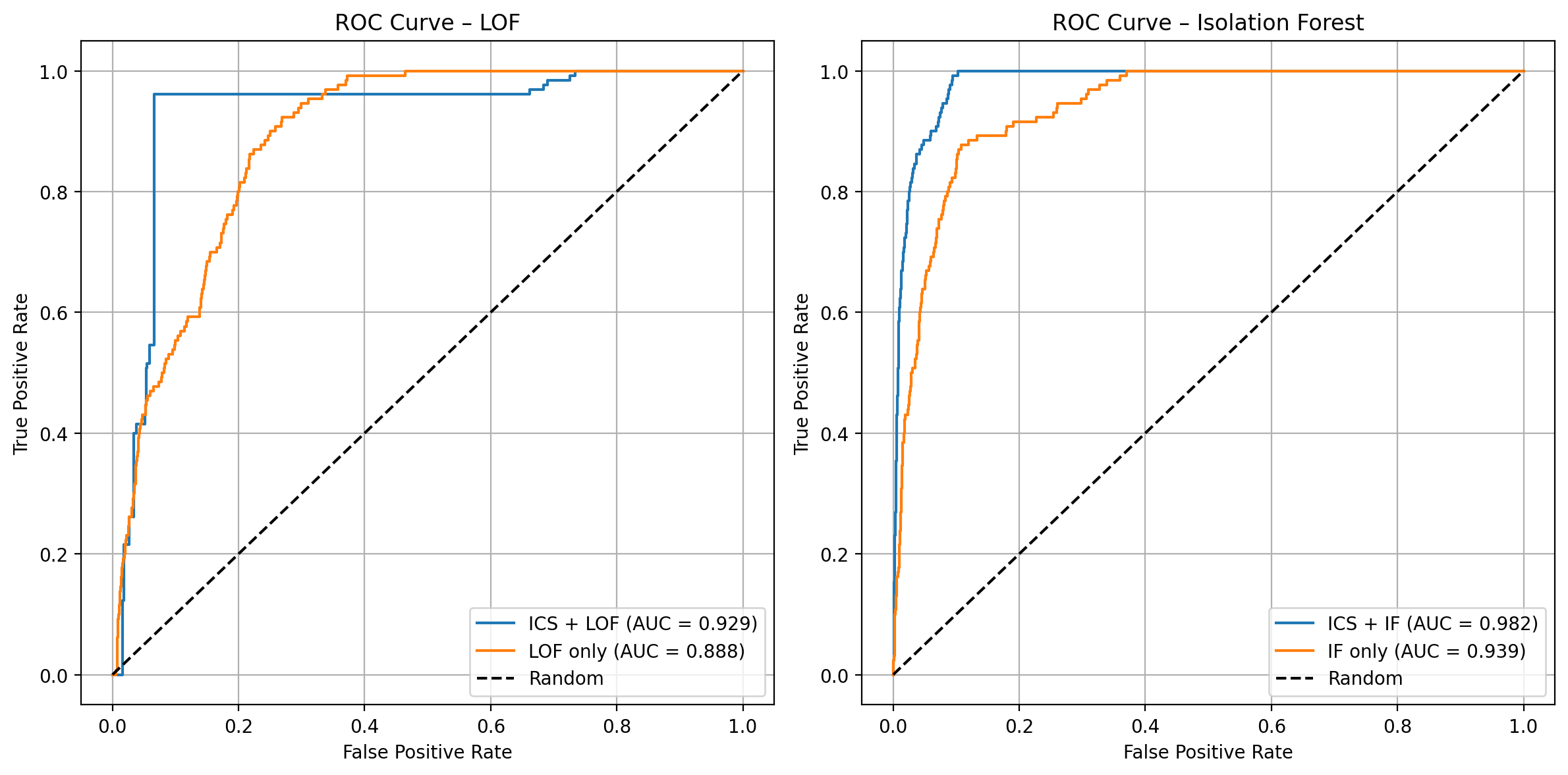
We compare the four methods with ROC curves, confusion matrices and F1 scores.

from sklearn.metrics import roc_curve, auc, confusion_matrix, ConfusionMatrixDisplay, f1_score
import matplotlib.pyplot as plt

# ROC curves

def plot_roc(ax, curves, title, y_test):
    for label, scores in curves.items():
        fpr, tpr, _ = roc_curve(y_test, scores)
        auc_val = auc(fpr, tpr)
        ax.plot(fpr, tpr, label=f"{label} (AUC = {auc_val:.3f})")
    ax.plot([0, 1], [0, 1], "k--", label="Random")
    ax.set_xlabel("False Positive Rate")
    ax.set_ylabel("True Positive Rate")
    ax.set_title(title)
    ax.legend()
    ax.grid(True)

fig, axes = plt.subplots(1, 2, figsize=(12, 6))

# Subplot 1 : LOF
plot_roc(ax=axes[0],
         curves={"ICS + LOF": scores_lof_ics, "LOF only": scores_lof_plain},
         title="ROC Curve – LOF",
         y_test=y_test)

# Subplot 2 : Isolation Forest
plot_roc(ax=axes[1],
         curves={"ICS + IF": scores_if_ics,  "IF only": scores_if_plain},
         title="ROC Curve – Isolation Forest",
         y_test=y_test)

plt.tight_layout()
plt.show()

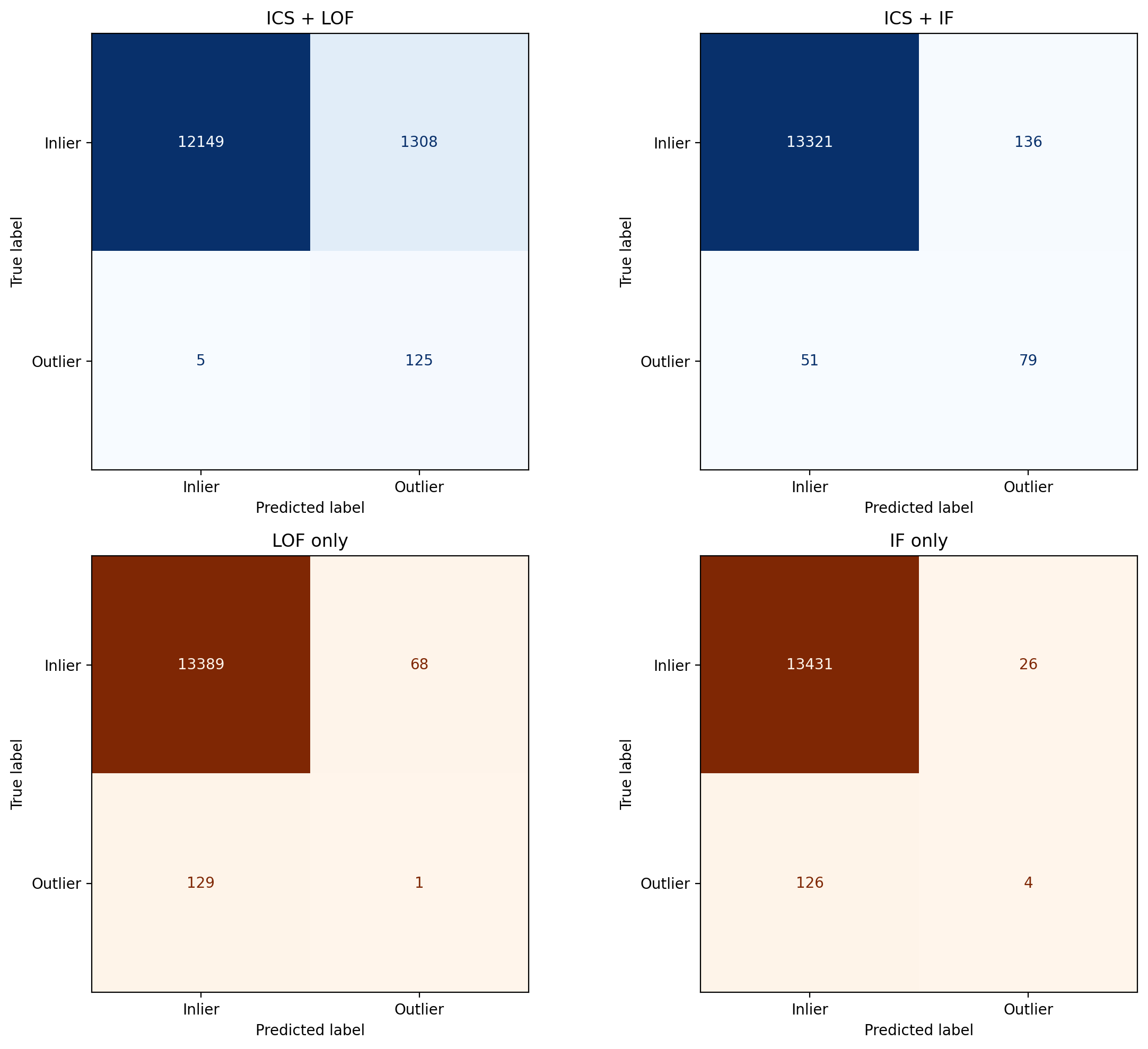
# Confusion matrices

def plot_confusion(ax, y_pred_bin, title, cmap):
    cm = confusion_matrix(y_test, y_pred_bin)
    ConfusionMatrixDisplay(cm, display_labels=["Inlier", "Outlier"]).plot(
        ax=ax, cmap=cmap, colorbar=False
    )
    ax.set_title(title)

fig, axes = plt.subplots(2, 2, figsize=(12, 10))

plot_confusion(ax=axes[0, 0], y_pred_bin=y_pred_ics_bin, title="ICS + LOF", cmap=plt.cm.Blues)
plot_confusion(ax=axes[1, 0], y_pred_bin=y_pred_plain_bin, title="LOF only", cmap=plt.cm.Oranges)
plot_confusion(ax=axes[0, 1], y_pred_bin=y_pred_if_ics_bin, title="ICS + IF", cmap=plt.cm.Blues)
plot_confusion(ax=axes[1, 1], y_pred_bin=y_pred_if_plain_bin, title="IF only", cmap=plt.cm.Oranges)

plt.tight_layout()
plt.show()

# F1 scores

f1_plain = f1_score(y_test, y_pred_plain_bin)
f1_ics = f1_score(y_test, y_pred_ics_bin)
f1_if_plain = f1_score(y_test, y_pred_if_plain_bin)
f1_if_ics = f1_score(y_test, y_pred_if_ics_bin)

print(f"F1 score LOF only: {f1_plain:.3f}")
print(f"F1 score ICS + LOF: {f1_ics:.3f}")
print(f"F1 score IF only: {f1_if_plain:.3f}")
print(f"F1 score ICS + IF: {f1_if_ics:.3f}")

F1 score LOF only: 0.010
F1 score ICS + LOF: 0.160
F1 score IF only: 0.050
F1 score ICS + IF: 0.458

Adding ICS as a pre-processing step improves the area under the curve (AUC) for both LOF and Isolation Forest analysis. However, due to the strong class imbalance, ROC curves may provide an overly optimistic view of performance. Precision-recall-oriented metrics such as the F1 score are more informative in this setting. It rises from 0.010 to 0.160 for LOF and from 0.050 to 0.458 for Isolation Forest. The confusion matrices further demonstrate that ICS helps to detect many more anomalies while only moderately increasing the number of false positives, particularly in the case of Isolation Forest.

Overall, these results suggest that ICS can greatly enhance the performance of anomaly detection methods on imbalanced datasets.