Circular structure example
This example is adapted from Caussinus et al. (2023), which is itself similar to Example 4.3 from Caussinus and Ruiz (1995).
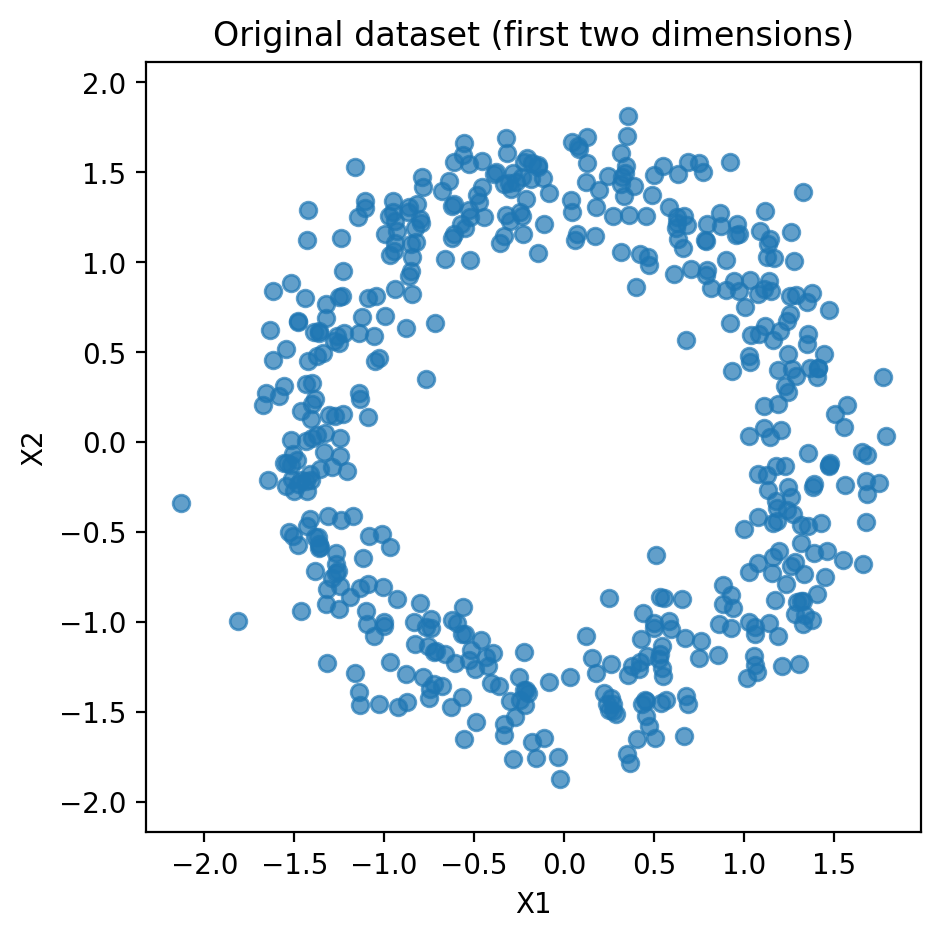
In the plane of the first two coordinates, points are generated according to a uniform distribution on the circle with centre \(0\) and radius \(sqrt(2)\). Noise is then added, following a normal distribution with \(p\) independent coordinates, variance \(σ^2\) on the first two components and \(1 + σ^2\) on the others.
import numpy as np
import matplotlib.pyplot as plt
from sklearn.decomposition import PCA
from sklearn.preprocessing import StandardScaler
from icspylab import ICS, cov, tcov
The example specifies \(p = 4\), \(σ = 0.2\) and \(n = 500\) points.
p = 4
sigma = 0.2
n = 500


def points_uniform_circle(n, p=2, rayon=np.sqrt(2)):
    x = np.random.normal(size=(n, p))
    norms = np.linalg.norm(x, axis=1, keepdims=True)
    return rayon * x / norms


# Generate the data

rng = np.random.default_rng(seed=0)

signal = points_uniform_circle(n, p=2, rayon=np.sqrt(2))

X1 = signal + rng.multivariate_normal(
    mean=np.zeros(2),
    cov=sigma**2 * np.eye(2),
    size=n
)

X2 = rng.multivariate_normal(
    mean=np.zeros(p-2),
    cov=(1 + sigma**2) * np.eye(p-2),
    size=n
)

X = np.hstack((X1, X2))

# Plot the original data
plt.figure(figsize=(5, 5))
plt.scatter(X[:, 0], X[:, 1], alpha=0.7)
plt.title("Original dataset (first two dimensions)")
plt.xlabel("X1")
plt.ylabel("X2")
plt.axis("equal")
plt.show()
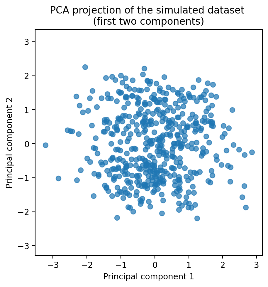
Given the way the data is simulated, the covariance matrix is of the form \((1 + σ^2)I\), so PCA results in arbitrary projections, as shown in the figure below.
# PCA
scaler = StandardScaler().set_output(transform="pandas")
X_scaled = scaler.fit_transform(X)
pca = PCA(n_components=2)
X_pca = pca.fit_transform(X_scaled)

# Plot PCA projection
plt.figure(figsize=(5, 5))
plt.scatter(X_pca[:, 0], X_pca[:, 1], alpha=0.7)
plt.title("PCA projection of the simulated dataset (first two components)")
plt.xlabel("Principal component 1")
plt.ylabel("Principal component 2")
plt.axis("equal")
plt.show()
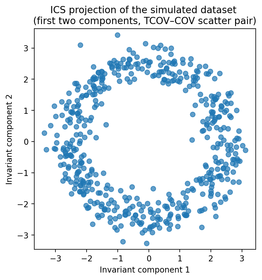
On the contrary, ICS enables the circular structure of the data to be recovered in the first two components.
# ICS
ics = ICS(S1="tcov", S2="cov", algorithm="standard")
X_ics = ics.fit_transform(X)

# Plot ICS projection
plt.figure(figsize=(5, 5))
plt.scatter(X_ics[:, 0], X_ics[:, 1], alpha=0.7)
plt.title("ICS projection of the simulated dataset \n(first two components, TCOV–COV scatter pair)")
plt.xlabel("Invariant component 1")
plt.ylabel("Invariant component 2")
plt.axis("equal")
plt.show()