Quick Start
This section provides examples of how to use the ICSpyLab package. The core of the package is the ICS class. The implementation is similar to the sklearn framework, including a fit-transform logic. For more information about the arguments and methods, check out the Module page.
Example 1: Fit and transform ICS
This first example shows how to instantiate an ICS object to compute the invariant components.
The output can be summarized using the icspylab.ics.ICS.describe() method.
import pandas as pd
from icspylab import ICS, cov, covW
from sklearn.datasets import load_iris

# Load dataset
iris = load_iris()
X = pd.DataFrame(iris.data, columns=iris.feature_names)

# Instantiate ICS object
ics = ICS() # default parameters

# Alternative instantiations (not shown):
ics_str = ICS(S1="cov", S2="cov4") # string values for S1 and S2
ics_args = ICS(S1=cov, S2=covW, algorithm="standard", S2_args={"alpha": 1, "cf": 2}) # custom arguments

# Fit and transform the ICS model (equivalent of the function ICS-S3() from the R package ICS)
X_new = ics.fit_transform(X)

# Printing a summary
ics.describe()
Example output:
ICS based on two scatter matrices:
S1: cov
S1_args: None
S2: cov4
S2_args: None

Information on the algorithm:
algorithm: eigh
center: False
fix_signs: scores

The generalized kurtosis measures of the components are:
IC_1: 1.2074
IC_2: 1.0269
IC_3: 0.9292
IC_4: 0.7405

Information on the component selection:
method_select: None
select_args: None
All components are kept: ['IC_1', 'IC_2', 'IC_3', 'IC_4']

The coefficient matrix of the linear transformation is:
     sepal length (cm) sepal width (cm) petal length (cm) petal width (cm)
IC_1       -0.52335      1.99326      2.37305     -4.43078
IC_2        0.83296      1.32750     -1.26665      2.78998
IC_3        3.05683     -2.22695     -1.63543      0.36544
IC_4        0.05244      0.60315     -0.34826     -0.37984
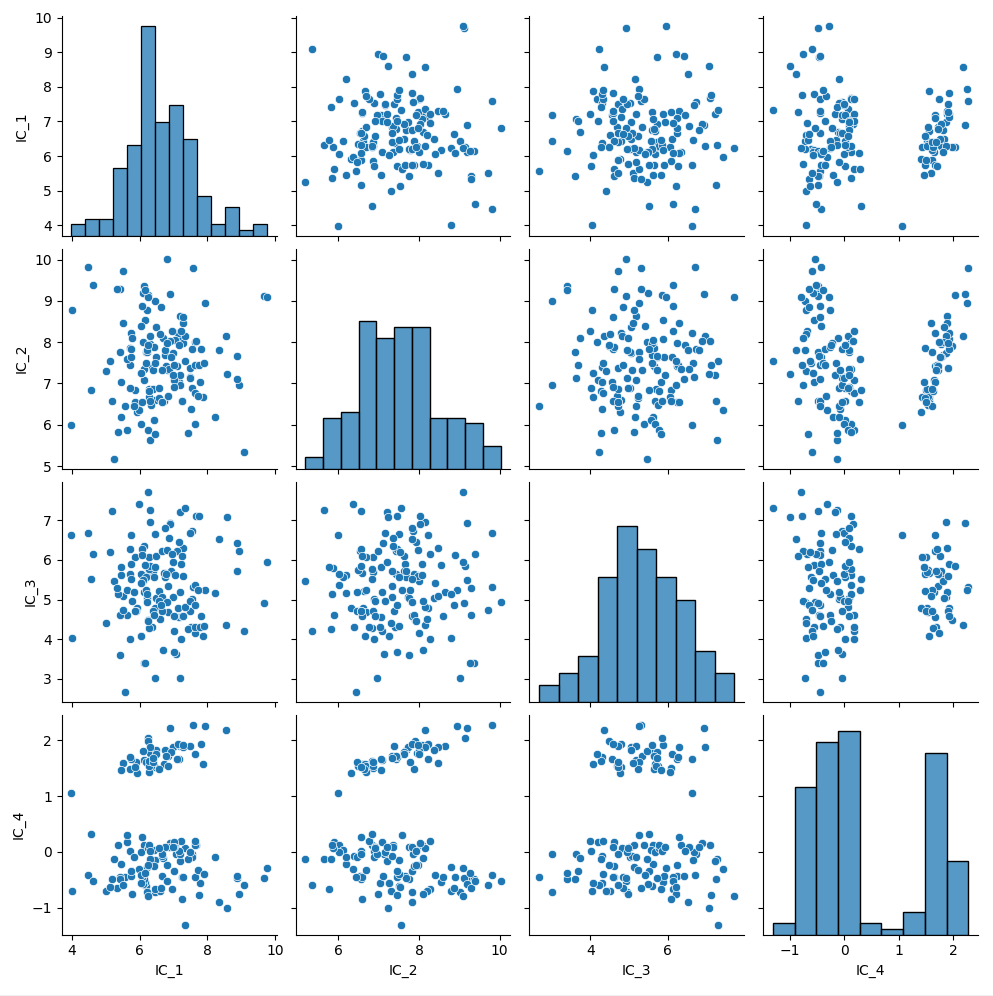
Example 2: Plotting functionalities
This example illustrates how to plot the transformed data (invariant components) using icspylab.plot.plot_ics(),
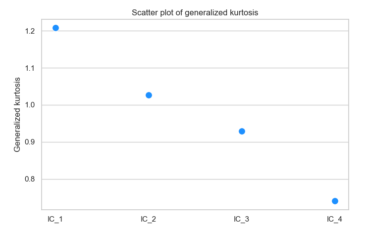
and the kurtosis of the invariant components (corresponding to the eigenvalues of the joint diagonalization problem)
using plot_kurtosis().
from icspylab import plot_ics

# Plot the invariant components
plot_ics(X_new)
Example plot:
# Plot kurtosis (eigenvalues)
ics.plot_kurtosis()
Example plot:
Example 3: Machine Learning pipeline
This example shows how to fit and transform separately, as is usually done in machine learning pipelines.
from sklearn.datasets import load_iris
from sklearn.model_selection import train_test_split
from sklearn.linear_model import LogisticRegression

# Load the Iris dataset
iris = load_iris()
X = iris.data
y = iris.target

# Split the data into training and test sets
X_train, X_test, y_train, y_test = train_test_split(X, y, test_size=0.2, random_state=42)

# Create a logistic regression model with ICS as a preprocessing step
ics = ICS()
model = LogisticRegression(max_iter=200)

# Train the model on the training set
ics.fit(X_train)
X_train_ics = ics.transform(X_train)
model.fit(X_train_ics, y_train)

# Make predictions on the test set
X_test_ics = ics.transform(X_test)
y_pred = model.predict(X_test_ics)