ICS principle
This tutorial explains the objective of the ICS method and builds intuition about how invariant components are computed. The explanation is based on a comparison with Linear Discriminant Analysis (LDA). Indeed, ICS can be interpreted as an unsupervised analogue of LDA, where class labels are not required.
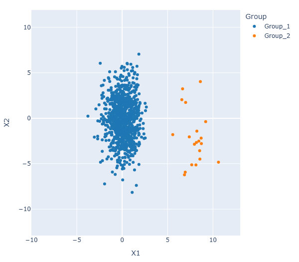
We begin by recalling the principle of LDA. Consider a dataset generated from a mixture of Gaussian distributions: a main bulk of observations and a smaller group located in another region of the space. In a clustering context, this example can be viewed as one large cluster and a smaller one. Alternatively, it can be interpreted as an anomaly detection problem, where the smaller group represents atypical observations.
import numpy as np
import pandas as pd

# Generate data

# Set parameters to generate data
n_samples = 980
n_outliers = 20
n_features = 2
add_outliers = True

# Generate Gaussian data of shape (125,2)
gen_cov = np.diag((1, 5))
gen_loc = np.array([0, 0])

X = np.random.default_rng().multivariate_normal(gen_loc, gen_cov, n_samples)
df = pd.DataFrame(X, columns=["X1", "X2"])
df["Group"] = "Group_1"

# Add some outliers
if add_outliers:
    outlier_cov = gen_cov
    outlier_loc = np.array([8, -2])
    X_out = np.random.default_rng().multivariate_normal(outlier_loc, outlier_cov, n_outliers)
    X = np.concatenate((X, X_out), axis=0)
    df_out = pd.DataFrame(X_out, columns=["X1", "X2"])
    df_out["Group"] = "Group_2"
    df = pd.concat([df, df_out])
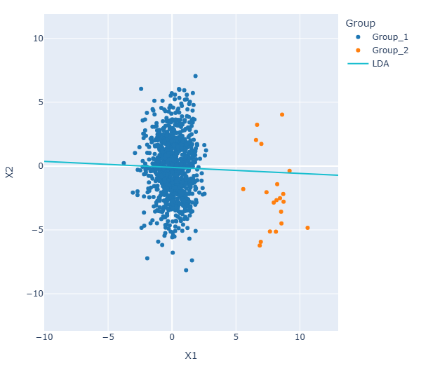
LDA aims to find a low-dimensional subspace that maximizes class separation, known as the Fisher discriminant subspace. This is achieved by maximizing the ratio of the between-class scatter matrix \(B\) to the within-class scatter matrix \(W\):
ICS also aims to identify a low-dimensional subspace that highlights the directions separating different groups of observations, but without using class labels. In that sense, ICS can be viewed as an unsupervised analogue of LDA, as it seeks to recover the Fisher discriminant subspace from the features alone.
Instead of relying on the between-class and within-class scatter matrices (that cannot be computed without the labels), ICS maximizes the contrast between two scatter matrices that capture different aspects of the data distribution. These matrices are required to be affine equivariant and positive definite.
Let \(Y\) be a random vector of dimension \(p\), with distribution function \(F_Y\). A scatter matrix of \(Y\), denoted \(V(F_Y)\), is a symmetric positive definite matrix of dimension \(p \times p\) and affine equivariant. Let \(\mathcal{P}_p\) be the set of all positive definite symmetric matrices of order \(p\).
ICS then solves a generalized eigenvalue problem of the form:
where \(V_1, V_2 \in \mathcal{P}_p\).
For instance, we can use:
The covariance matrix \(\mathrm{COV}\), which measures overall dispersion, as \(V_1\).
The fourth-moment scatter matrix \(\mathrm{COV}_4\), which emphasizes directions associated with deviations from Gaussianity, as \(V_2\).
These two scatters are given by
and
where \(d^2\) is the square of the Mahalanobis distance:
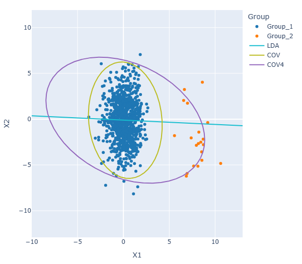
In the plot below, \(\mathrm{COV}\) can be viewed as analogous to the within-class scatter in LDA, since it captures the global variability of the data. In contrast, \(\mathrm{COV}_4\) gives more weight to directions associated with group separation, playing a role similar to a between-class scatter.
To compute the invariant components, ICS relies on the joint diagonalization of \(V_1\) and \(V_2\).
where \(V_1, V_2 \in \mathcal{P}_p\), \(\Delta = \text{diag}(\rho_1, \dots, \rho_p)\), \(\rho_1, \dots, \rho_p\) being the eigenvalues of \(V_1^{-1}V_2\) sorted in descending order, and \(H = (h_1, \dots, h_p)\) is a matrix containing the corresponding eigenvectors.
The components are given by
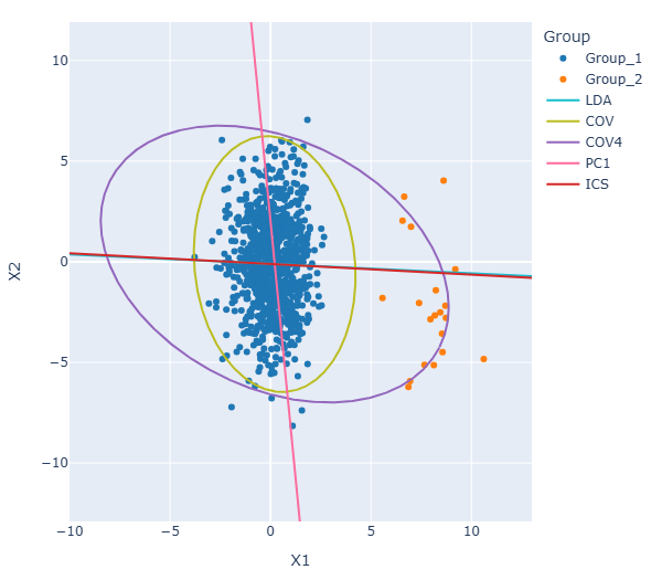
The first invariant component is shown in the plot below. Its direction is very close to that obtained with LDA, illustrating how ICS can recover the Fisher discriminant subspace in this example. For comparison, the first principal component is also displayed. This direction is substantially different and does not provide a projection that clearly separates the two groups, highlighting the limitation of variance-based dimension reduction in this setting.
References
Caussinus, H., & Ruiz, A. (1990). Interesting projections of multidimensional data by means of generalized principal component analyses. In Compstat: Proceedings in Computational Statistics, 9th Symposium held at Dubrovnik, Yugoslavia, 1990 (pp. 121–126). Heidelberg: Physica-Verlag HD. https://link.springer.com/chapter/10.1007/978-3-642-50096-1_19.
Tyler, D.E., Critchley, F., Dümbgen, L., and Oja, H. (2009), Invariant coordinate selection, Journal of the Royal Statistical Society, Series B, 71, 549-592. https://doi.org/10.1111/j.1467-9868.2009.00706.x.