Custom Component Selection
In this section, “component selection” refers to the optional step performed after the ICS transformation to
retain only a subset of invariant coordinates.
While some methods are already available in ICSpyLab, this section illustrates how to use a custom method to select
the invariant components. As we will see, the method_select parameter allows users to inject a component
selection strategy directly into the ICS fitting procedure.
We start start with some data exploration, we apply ICS with the scatter pair COV-COV4 on the Iris dataset.
By default, method_select = None and all invariant components are kept.
import pandas as pd
from icspylab import ICS, ComponentSelect, plot_ics
from sklearn.datasets import load_iris

# Load dataset
iris = load_iris()
X = pd.DataFrame(iris.data, columns=iris.feature_names)

# Instantiate ICS object
ics = ICS(S1="cov", S2="cov4", algorithm="standard")

# Fit and transform the ICS model
X_ics = ics.fit_transform(X)
plot_ics(X_ics)
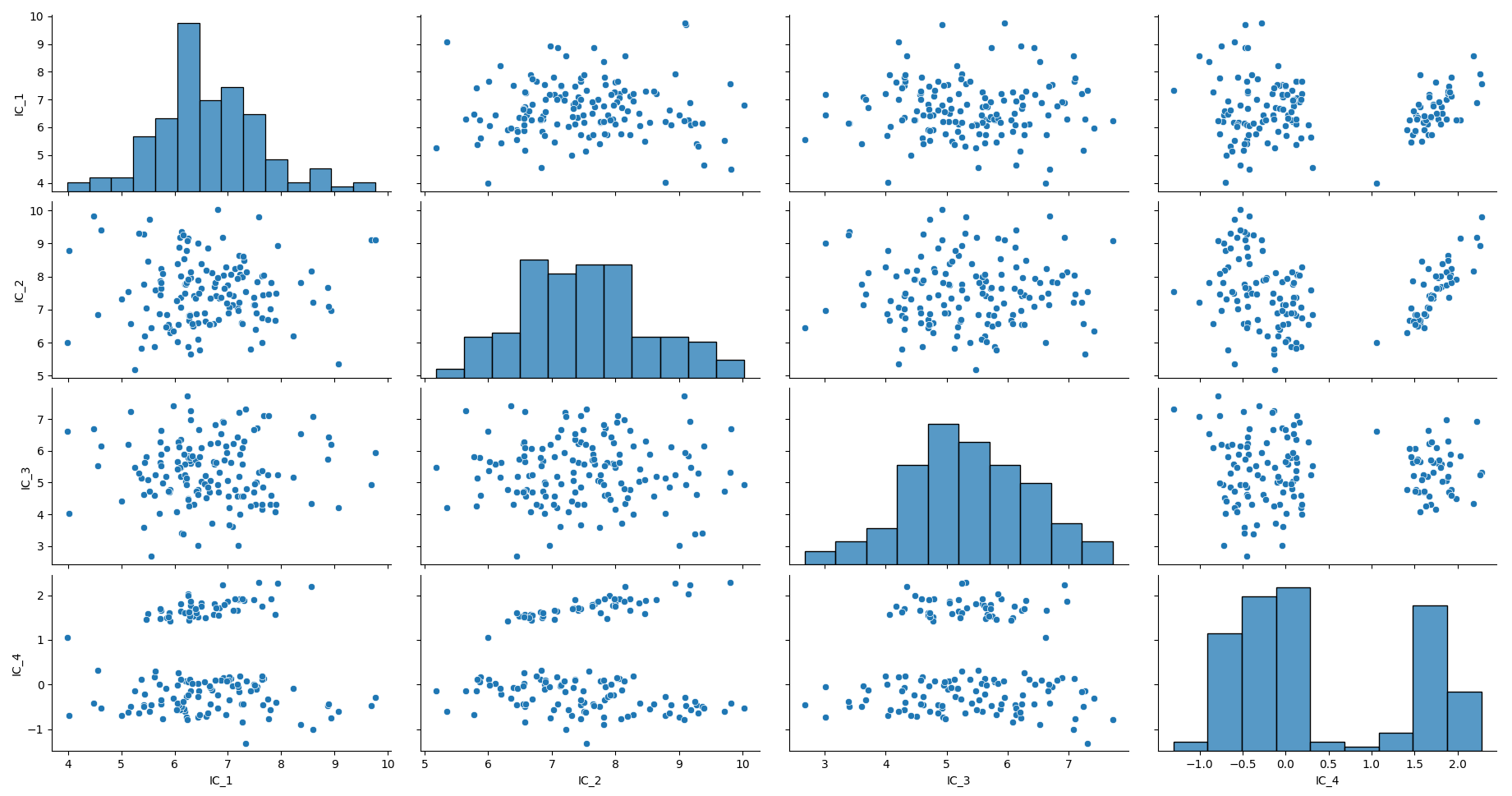
Looking at the invariant coordinates on the plot above, you decide that you want to keep only the last component.
If you just need a one-shot usage you can simply apply the selection method on the output X_ics.
# Keep the last component only
X_ics_reduced = X_ics[:, -1]
print("Shape after ICS and manual component selection:", X_ics_reduced.shape)
Shape after ICS and manual component selection: (150,)
While manual slicing of X_ics is sufficient for exploratory analysis, integrating the selection step into the ICS
estimator is recommended when building pipelines or performing model selection. To do so, recall that the method_select
parameter of an ICS instance is
(if not None) a callable returning a ComponentSelect object.
The ComponentSelect object acts as a container describing which invariant components are retained and how they map
back to the original feature space. Each ComponentSelect has the
following attributes: label,
components,
n_components,
component_names,
info.
After the component computation, during the component selection step of the ICS fit() method,
method_select is called with the following parameters:
X(ndarray): Data to fit the ICS model, where rows are samples and columns are features.W(ndarray): Transformation matrix in which each row contains the coefficients of the linear transformation to the corresponding invariant coordinate.kurtosis(ndarray): Generalized kurtosis values.skewness(ndarray): Skewness values.**select_args: Other arguments from the parameterselect_argsof theICSobject.
The method to select the last component is then:
def select_last_comp(W, **kwargs):
    all_comp_names = [f"IC_{i + 1}" for i in range(W.shape[1])]
    p = W.shape[1]
    selected_component_names = all_comp_names[-1:]

    # Keep only the selected components
    name_to_idx = {name: i for i, name in enumerate(all_comp_names)}
    idx = [name_to_idx[name] for name in selected_component_names]
    components = W[idx, :]
    n_components = len(selected_component_names)

    return ComponentSelect(label="custom", components=components, n_components=n_components,
                           component_names=selected_component_names, info=None)
Recall that each row of W corresponds to one invariant component, expressed in the original feature space.
Do not forget **kwargs for consistency! The **kwargs argument ensures forward compatibility and allows the function to
receive additional information such as kurtosis, skewness, or user-defined parameters without breaking the API.
Lets try it on the Iris dataset:
# Instantiate ICS object
ics_custom = ICS(S1="cov", S2="cov4", algorithm="standard", method_select=select_last_comp)

# Fit and transform the ICS model
X_ics_custom = ics_custom.fit_transform(X)

print(f"Shape after ICS with select_last_comp: {X_ics_custom.shape}"
      f" with component names: {ics_custom.component_names_}")
Shape after ICS with select_last_comp: (150, 1) with component names: ['IC_4']
Finally, you want to keep some flexibility and select the last q components (default is q=1).
def select_last_q_comp(W, q=1, **kwargs):
    all_comp_names = [f"IC_{i + 1}" for i in range(W.shape[1])]
    p = W.shape[1]
    selected_component_names = all_comp_names[-q:]

    # Keep only the selected components
    name_to_idx = {name: i for i, name in enumerate(all_comp_names)}
    idx = [name_to_idx[name] for name in selected_component_names]
    components = W[idx, :]
    n_components = len(selected_component_names)

    return ComponentSelect(label="custom", components=components, n_components=n_components,
                           component_names=selected_component_names, info=None)
# Instantiate ICS object with select_last_q_comp and default parameters
ics_custom = ICS(S1="cov", S2="cov4", algorithm="standard", method_select=select_last_q_comp)

# Fit and transform the ICS model
X_ics_custom = ics_custom.fit_transform(X)

print(f"Shape after ICS with select_last_q_comp (default q): {X_ics_custom.shape}"
      f" with component names: {ics_custom.component_names_}")
Shape after ICS with select_last_q_comp (default q): (150, 1) with component names: ['IC_4']
We have the same result as q=1 is the default value.
Additional parameters can be passed to the selection function via the select_args dictionary of the ICS estimator.
To select the last 2 components, just specify q=2 in select_args.
# Instantiate ICS object with select_last_q_comp and q=2
ics_custom = ICS(S1="cov", S2="cov4", algorithm="standard", method_select=select_last_q_comp, select_args={"q": 2})

# Fit and transform the ICS model
X_ics_custom = ics_custom.fit_transform(X)

print(f"Shape after ICS with select_last_q_comp (q=2): {X_ics_custom.shape}"
      f" with component names: {ics_custom.component_names_}")
Shape after ICS with select_last_q_comp (q=2): (150, 2) with component names: ['IC_3', 'IC_4']
This approach allows users to seamlessly integrate custom component selection strategies into ICS while remaining fully compatible with scikit-learn pipelines.